Automated high-throughput Wannierisation#
In the following tutorial you will learn how to perform automated high-throughput Wannierisation using a dedicated AiiDA workchain.
The protocol for automating the construction of Wannier functions is discussed in the following article:
Valerio Vitale, Giovanni Pizzi, Antimo Marrazzo, Jonathan Yates, Nicola Marzari, Arash Mostofi, Automated high-throughput wannierisation, npj Computational Materials (2020); https://www.nature.com/articles/s41524-020-0312-y https://arxiv.org/abs/1909.00433
whose data is available on the Materials Cloud Archive as:
Valerio Vitale, Giovanni Pizzi, Antimo Marrazzo, Jonathan R. Yates, Nicola Marzari, Arash A. Mostofi, Automated high-throughput Wannierisation, Materials Cloud Archive (2019), doi: 10.24435/materialscloud:2019.0044/v2.
The protocol leverages the SCDM method introduced in:
Anil Damle, Lin Lin, and Lexing Ying, Compressed representation of kohn–sham orbitals via selected columns of the density matrix Journal of Chemical Theory and Computation 11, 1463–1469 (2015).
Anil Damle and Lin Lin, Disentanglement via entanglement: A unified method for wannier localization, Multiscale Modeling & Simulation 16, 1392–1410 (2018).
The initial workflow was written by Antimo Marrazzo (EPFL) and Giovanni Pizzi (EPFL) (and is available, in a Virtual Machine, on the Materials Cloud entry mentioned above). It was later substantially improved and upgraded to AiiDA v1.x by Junfeng Qiao (EFPL). The SCDM implementation in Quantum ESPRESSO was done by Valerio Vitale (Imperial College London and University of Cambridge).
Note
Launch while you read! The workflow should take a few minutes to run on the virtual machine (5-10 minutes). So, we suggest that you launch it now (following the suggestions below) in the background, while you read through the tutorial.
Preparation#
You can download the launch script for the workflow here: launch_wannier.py.
The script accepts one argument, which is the location of the crystal structure file (in XSF format) for which you want to run the Wannierisation.
As an example, you can pick any one of the simple crystal structures from this list below:
Once you downloaded both the launcher script and one of the XSF files, first adapt the launcher script content, as usual, filling in the names of the codes that you want to use.
Then, launch the script with the following command:
runaiida launch_wannier.py CsH.xsf
(in the following, we will use CsH as an example); you can replace CsH.xsf with any other structure of the list above, e.g. PtS2.xsf, or GaAs.xsf, …
Introduction#
The use of maximally-localised Wannier functions (MLWFs) in high-throughput (HT) workflows has been hindered by the fact that generating MLWFs automatically and robustly without any user intervention and for arbitrary materials is, in general, very challenging.
The procedure to obtain MLWFs requires to specify a number of parameters that depends on the specific system under study, such as
the type of projections to build the \(A_{mn}({\mathbf{k}})\) matrix
and, in the case of entangled bands, many other parameters like
the number of Wannier functions,
the frozen energy window,
the outer energy window, …
The SCDM method allows to circumvent the need to specify initial projections, by introducting an algorithm that builds the \(A_{mn}({\mathbf{k}})\) matrix by optimally selecting columns of the density matrix \(P_{\mathbf{k}}\)
where \(f(\epsilon_{n\mathbf{k}})\) is an occupation function.
The SCDM algorithm is based on a QR factorization with column pivoting (QRCP) and it is
currently implemented in the pw2wannier90.x code of Quantum Espresso.
It is worth to stress that the occupation function does not necessarily correspond to a physical smearing, but it is used as a “window function” that restricts the manifold to the energy region of interest. For example, the isolated-band case can be recovered by setting \(f(\epsilon_{n\mathbf{k}})=1\) for energy values \(\epsilon_{n\mathbf{k}}\) within the energy range of the isolated bands, and zero elsewhere.
Another typical choice for the occupation function is the so-called complementary error function (erfc)
and it is used to to deal with a manifold of bands that are entangled only in the upper energy region (e.g. for metals, or for the conduction band of insulators). Another possible choice for the occupation function could be a Gaussian, for instance to extract bands in a specific energy range from a fully entangled manifold.
While the SCDM method allows to avoid the disentanglement procedure, and so the need to specify the frozen and outer window, it does not provide a recipe to set the smearing function parameters \(\mu\) and \(\sigma\). In addition, the number of Wannier functions remains to be set and a sensible value typically requires some chemical consideration, such as counting the number of atomic orbitals of a given orbital character (e.g. \(s\), \(p\), \(d\), \(sp^3\), …).
The Wannier90BandsWorkChain (distributed in the aiida-wannier90-workflows package) is an AiiDA workchain that implements a protocol that deals with the choice
of the number of Wannier functions and sets the parameters \(\mu\) and \(\sigma\) defining
the smearing function. For a full explanation of the protocol we refer to the article
Automated high-throughput wannierisation, while here we
just outline the main features.
The workflow starts by running a DFT calculation (with Quantum ESPRESSO) using automated workchains distributed within the aiida-quantumespresso plugin, that take care of automation for the calculations performed with Quantum ESPRESSO (QE). This is followed by a calculation of the projectability, that is the projection of the Kohn-Sham states onto localised atomic orbitals:
where the \(\phi_{Ilm}(\mathbf{k})\) are the pseudo-atomic orbitals (PAO) employed in the generation of the pseudopotentials, \(I\) is an index running over the atoms in the cell and \(lm\) define the usual angular momentum quantum numbers.
The workflow is designed for the specific use case where we are interested in Wannierising the occupied bands (plus, optionally, some unoccupied or partially occupied bands) in insulators and in metals.
The number of Wannier functions is automatically set equal to the number of PAOs defined in the pseudopotentials (and the pseudopotentials are automatically taken from the SSSP efficiency library).
The projectabilities on these PAO orbitals are then computed and used to
set the optimal smearing function (erfc) parameters \(\mu\) and \(\sigma\), as explained in the paper
Automated high-throughput wannierisation.
After the calculation of the projectabilities, the workflow proceeds with the usual Wannierisation step: first
it computes the overlap and projection matrices using pw2wannier90, and then it runs the Wannier90 code.
Here we summarise the main steps of the Wannier90BandsWorkChain:
SCF (QuantumESPRESSO
pw.x)NSCF (QuantumESPRESSO
pw.x)Projectability (QuantumESPRESSO
projwfc.x)Wannier90 pre-processing (
wannier90.x -pp)Overlap matrices \(M_{mn}\), initial projections with SCDM \(A_{mn}\) (QuantumESPRESSO
pw2wannier90.x)Wannierisation (
wannier90.x)
The output of the workflow includes several nodes, among which the projectabilities and interpolated band structure, that we are going to inspect after the run.
Running the workflow#
If you have not launch the script yet, please do it now!
Here we focus on how to run the Wannier90BandsWorkChain, the AiiDA workchain
that implements the automation workflow to obtain MLWFs.
Important note: For this tutorial, in order to keep the total simulation time down to ~5-10 minutes on a typical laptop, we run the workflow using the fast protocol, where some of the parameters are reduced to
speed up the calculations (with respect to the converged
and tested parameters). For production please use the moderate protocol or precise.
We remind you that, to get a list of all the AiiDA processes (including calculations and workchains) that are running and their status you can use:
verdi process list
or alternatively
verdi process list -p 1 -a
to see all workflows and calculations, even completed, that have been launched in the past 1 day.
Since you have already run the workflow by now, run the commands above to retrieve the corresponding PKs.
Here is the script that you have run:
#!/usr/bin/env runaiida
import os
import sys

from ase.io import read as aseread

from aiida import orm
from aiida.engine import submit

from aiida_wannier90_workflows.workflows import Wannier90BandsWorkChain

# Code labels for `pw.x`, `pw2wannier90.x`, `projwfc.x`, and `wannier90.x`.
# Change these according to your aiida setup.
codes = {
    "pw": "qe-pw-6.8@localhost",
    "projwfc": "qe-projwfc-6.8@localhost",
    "pw2wannier90": "qe-pw2wannier90-6.8@localhost",
    "wannier90": "wannier90-3.1@localhost",
}

# Filename of a structure.
# filename = "GaAs.xsf"
if len(sys.argv) != 2:
    print(f"Please pass a filename for a structure as the argument.")
    sys.exit(1)
filename = sys.argv[1]
if not os.path.exists(filename):
    print(f"{filename} not existed!")
    sys.exit(1)

# Read a structure file and store as an `orm.StructureData`.
structure = orm.StructureData(ase=aseread(filename))
structure.store()
print(f"Read and stored structure {structure.get_formula()}<{structure.pk}>")

# Prepare the builder to launch the workchain.
# We use fast protocol to converge faster.
builder = Wannier90BandsWorkChain.get_builder_from_protocol(
    codes,
    structure,
    protocol="fast",
)

# Submit the workchain.
workchain = submit(builder)
print(f"Submitted {workchain.process_label}<{workchain.pk}>")

print(
    "Run any of these commands to check the progress:\n"
    f"verdi process report {workchain.pk}\n"
    f"verdi process show {workchain.pk}\n"
    "verdi process list\n"
)
Inspect the script in detail now, and make sure that you understand all its parts. The comments should guide you through it. As you will notice, the amount of information to provide to the workflow is really minimal: just the codes to use, the crystal structure, and the protocol.
Analyzing the outputs of the workflow#
Now we analyse the reports and outputs of the workflow using the command line.
When the Wannier90BandsWorkChain is running, or after its completion,
you can monitor its progress by
looking at its “report”, using the command
verdi process report <PK>
where <PK> corresponds to the workchain PK. You will see a list of log with messages produced by the workchain,
including the PKs of all its sub-workchains and of the calculations launched by the Wannier90BandsWorkChain.
The report will be similar to the following:
2022-05-12 22:07:11 [179 | REPORT]: [446|Wannier90BandsWorkChain|run_seekpath]: launching seekpath: CsH -> CsH
2022-05-12 22:07:11 [180 | REPORT]: [446|Wannier90BandsWorkChain|run_scf]: launching PwBaseWorkChain<454> in scf mode
2022-05-12 22:07:12 [181 | REPORT]:   [454|PwBaseWorkChain|run_process]: launching PwCalculation<459> iteration #1
2022-05-12 22:07:55 [182 | REPORT]:   [454|PwBaseWorkChain|results]: work chain completed after 1 iterations
2022-05-12 22:07:55 [183 | REPORT]:   [454|PwBaseWorkChain|on_terminated]: remote folders will not be cleaned
2022-05-12 22:07:55 [184 | REPORT]: [446|Wannier90BandsWorkChain|run_nscf]: launching PwBaseWorkChain<466> in nscf mode
2022-05-12 22:07:56 [185 | REPORT]:   [466|PwBaseWorkChain|run_process]: launching PwCalculation<469> iteration #1
2022-05-12 22:19:39 [187 | REPORT]:   [466|PwBaseWorkChain|results]: work chain completed after 1 iterations
2022-05-12 22:19:40 [188 | REPORT]:   [466|PwBaseWorkChain|on_terminated]: remote folders will not be cleaned
2022-05-12 22:19:40 [189 | REPORT]: [446|Wannier90BandsWorkChain|run_projwfc]: launching ProjwfcBaseWorkChain<476>
2022-05-12 22:19:40 [190 | REPORT]:   [476|ProjwfcBaseWorkChain|run_process]: launching ProjwfcCalculation<477> iteration #1
2022-05-12 22:19:50 [191 | REPORT]:   [476|ProjwfcBaseWorkChain|results]: work chain completed after 1 iterations
2022-05-12 22:19:50 [192 | REPORT]:   [476|ProjwfcBaseWorkChain|on_terminated]: remote folders will not be cleaned
2022-05-12 22:19:50 [193 | REPORT]: [446|Wannier90BandsWorkChain|run_wannier90_pp]: launching Wannier90BaseWorkChain<487> in postproc mode
2022-05-12 22:19:51 [194 | REPORT]:   [487|Wannier90BaseWorkChain|run_process]: launching Wannier90Calculation<489> iteration #1
2022-05-12 22:19:59 [195 | REPORT]:   [487|Wannier90BaseWorkChain|results]: work chain completed after 1 iterations
2022-05-12 22:19:59 [196 | REPORT]:   [487|Wannier90BaseWorkChain|on_terminated]: remote folders will not be cleaned
2022-05-12 22:20:00 [197 | REPORT]: [446|Wannier90BandsWorkChain|run_pw2wannier90]: launching Pw2wannier90BaseWorkChain<495>
2022-05-12 22:20:02 [198 | REPORT]:   [495|Pw2wannier90BaseWorkChain|run_process]: launching Pw2wannier90Calculation<497> iteration #1
2022-05-12 22:20:39 [199 | REPORT]:   [495|Pw2wannier90BaseWorkChain|results]: work chain completed after 1 iterations
2022-05-12 22:20:39 [200 | REPORT]:   [495|Pw2wannier90BaseWorkChain|on_terminated]: remote folders will not be cleaned
2022-05-12 22:20:40 [201 | REPORT]: [446|Wannier90BandsWorkChain|run_wannier90]: launching Wannier90BaseWorkChain<506>
2022-05-12 22:20:41 [202 | REPORT]:   [506|Wannier90BaseWorkChain|run_process]: launching Wannier90Calculation<508> iteration #1
2022-05-12 22:21:00 [203 | REPORT]:   [506|Wannier90BaseWorkChain|results]: work chain completed after 1 iterations
2022-05-12 22:21:00 [204 | REPORT]:   [506|Wannier90BaseWorkChain|on_terminated]: remote folders will not be cleaned
2022-05-12 22:21:00 [205 | REPORT]: [446|Wannier90BandsWorkChain|results]: Wannier90BandsWorkChain successfully completed
2022-05-12 22:21:01 [206 | REPORT]: [446|Wannier90BandsWorkChain|on_terminated]: remote folders will not be cleaned
Once the workchain has finished to run, you can look at all its inputs and outputs with
verdi node show <PK>
You should obtain an output similar to what follows:
Property     Value
-----------  ------------------------------------
type         Wannier90BandsWorkChain
state        Finished [0]
pk           446
uuid         c1106d99-8ff1-4ef0-ba6c-08fe69aa05eb
label
description
ctime        2022-05-12 22:07:09.484260+00:00
mtime        2022-05-12 22:21:01.119854+00:00
computer     [1] localhost

Inputs                             PK    Type
---------------------------------  ----  -------------
nscf
    pw
        pseudos
            Cs                     54    UpfData
            H                      25    UpfData
        code                       336   Code
        parameters                 430   Dict
    kpoints_force_parity           431   Bool
    kpoints                        432   KpointsData
    max_iterations                 433   Int
projwfc
    projwfc
        code                       337   Code
        parameters                 434   Dict
    max_iterations                 435   Int
pw2wannier90
    pw2wannier90
        code                       338   Code
        parameters                 436   Dict
    max_iterations                 437   Int
    scdm_sigma_factor              438   Float
scf
    pw
        pseudos
            Cs                     54    UpfData
            H                      25    UpfData
        code                       336   Code
        parameters                 426   Dict
    kpoints_distance               427   Float
    kpoints_force_parity           428   Bool
    max_iterations                 429   Int
wannier90
    wannier90
        code                       92    Code
        kpoints                    432   KpointsData
        parameters                 439   Dict
        settings                   440   Dict
    shift_energy_windows           441   Bool
    auto_energy_windows            442   Bool
    auto_energy_windows_threshold  443   Float
    max_iterations                 444   Int
clean_workdir                      445   Bool
structure                          425   StructureData

Outputs                 PK    Type
----------------------  ----  --------------
nscf
    output_band         472   BandsData
    output_parameters   474   Dict
    output_trajectory   473   TrajectoryData
    remote_folder       470   RemoteData
    retrieved           471   FolderData
projwfc
    Dos                 483   XyData
    bands               482   BandsData
    output_parameters   480   Dict
    projections         481   ProjectionData
    remote_folder       478   RemoteData
    retrieved           479   FolderData
pw2wannier90
    output_parameters   500   Dict
    remote_folder       498   RemoteData
    retrieved           499   FolderData
scf
    output_band         462   BandsData
    output_parameters   464   Dict
    output_trajectory   463   TrajectoryData
    remote_folder       460   RemoteData
    retrieved           461   FolderData
wannier90
    interpolated_bands  511   BandsData
    output_parameters   512   Dict
    remote_folder       509   RemoteData
    retrieved           510   FolderData
wannier90_pp
    nnkp_file           492   SinglefileData
    output_parameters   493   Dict
    remote_folder       490   RemoteData
    retrieved           491   FolderData
band_structure          511   BandsData
primitive_structure     450   StructureData
seekpath_parameters     448   Dict

Called                         PK  Type
---------------------------  ----  ---------------------------
seekpath_structure_analysis   447  seekpath_structure_analysis
scf                           454  PwBaseWorkChain
nscf                          466  PwBaseWorkChain
projwfc                       476  ProjwfcBaseWorkChain
wannier90_pp                  487  Wannier90BaseWorkChain
pw2wannier90                  495  Pw2wannier90BaseWorkChain
wannier90                     506  Wannier90BaseWorkChain

Log messages
---------------------------------------------
There are 9 log messages for this calculation
Run 'verdi process report 446' to see them
Analyzing and comparing the band structure#
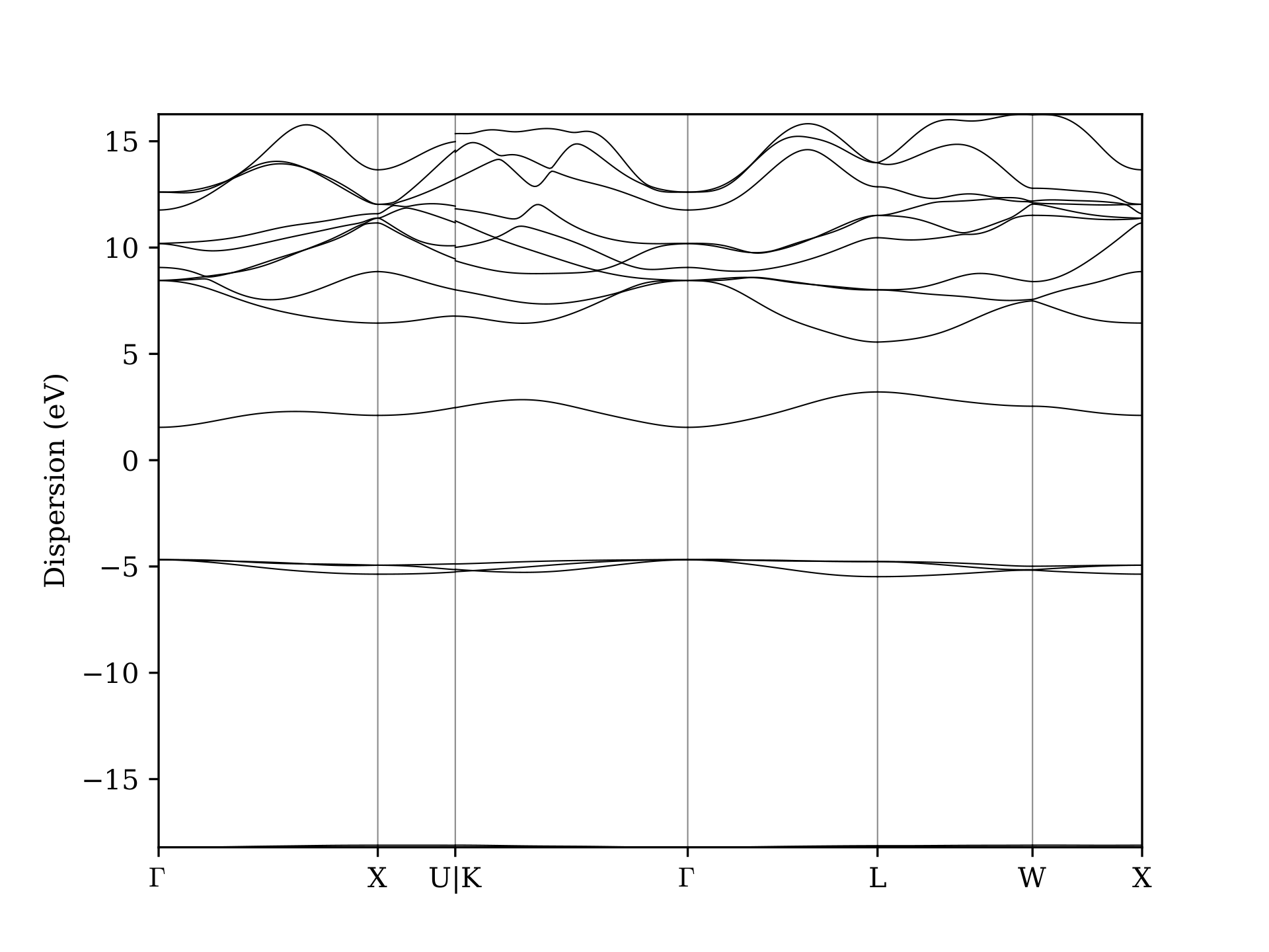
First let’s give a look at the interpolated band structure by exporting it to a PDF file with
verdi data bands export --format mpl_pdf --output band_structure.pdf <PK_bands>
where <PK_bands> stands for the BandsData PK produced by the workflow.
You can find it from the output of the verdi node show <PK> command
that you run before.
You should obtain a PDF like the following:
Now we compare the Wannier-interpolated bands with the full DFT bands calculation.
You can download the launch script for the DFT bands here: launch_pwbands.py.
Note we have a common interface for Wannier90BandsWorkChain and PwBandsWorkChain: we only need very minimal changes to calculate Wannier or DFT band structures.
#!/usr/bin/env runaiida
import os
import sys

from ase.io import read as aseread

from aiida import orm
from aiida.engine import submit

from aiida_quantumespresso.workflows.pw.bands import PwBandsWorkChain

# Code labels for `pw.x`
# Change these according to your aiida setup.
code = "qe-pw-6.8@localhost"

# Filename of a structure.
# filename = "GaAs.xsf"
if len(sys.argv) != 2:
    print(f"Please pass a filename for a structure as the argument.")
    sys.exit(1)
filename = sys.argv[1]
if not os.path.exists(filename):
    print(f"{filename} not existed!")
    sys.exit(1)

# Read a structure file and store as an `orm.StructureData`.
structure = orm.StructureData(ase=aseread(filename))
structure.store()
print(f"Read and stored structure {structure.get_formula()}<{structure.pk}>")

# Prepare the builder to launch the workchain.
# We use fast protocol to converge faster.
builder = PwBandsWorkChain.get_builder_from_protocol(
    code,
    structure,
    protocol="fast",
)
builder.pop("relax", None)

# Submit the workchain.
workchain = submit(builder)
print(f"Submitted {workchain.process_label}<{workchain.pk}>")

print(
    "Run any of these commands to check the progress:\n"
    f"verdi process report {workchain.pk}\n"
    f"verdi process show {workchain.pk}\n"
    "verdi process list\n"
)
For comparison, now we launch a DFT bands workchain
runaiida launch_pwbands.py CsH.xsf
To compare DFT and Wannier bands, run
aiida-wannier90-workflows plot bands <PwBandsWorkChain_PK> <Wannier90BandsWorkChain_PK>
This will show a figure like this
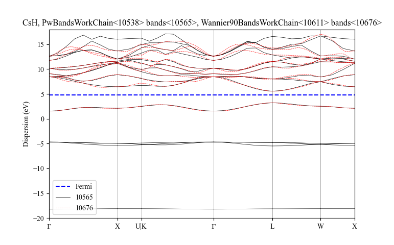
Note the semicore states are auto excluded by the workchain.
The Wannier band is different from DFT since we used the fast protocol. When using the default moderate protocol (will use more converged input parameters, and take more time to finish), we will get a more accurate band interpolation,
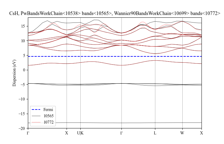
We can also compare bands using xmgrace.
For convenience, we have already computed for you all the full DFT band structures for all the
compounds for which we provided the XSF above (even if you could easily recompute these band structures using
the plugins and workflows included in the aiida-quantumespresso package). You can download the full DFT bands in xmgrace format (.agr) form this list:
In particular, taking CsH as an example, you can first export the Wannier-interpolated bands that you just computed earlier in xmgrace format with
verdi data bands export --format agr --output CsH_wan_bands.agr <PK_bands>
and then you can compare them with the full DFT band structure using xmgrace typing:
xmgrace CsH_dft_bands.agr CsH_wan_bands.agr
where you can replace CsH with the correct chemical formula of the crystal structure that you used.
For reference, here are the two xmgrace files for CsH:
CsH_dft_bands.agr
CsH_wan_bands.agr.
In the case of CsH, you should obtain something like the following plot (note that we slightly updated the colors and graphical appearance of the plot with respect to the default one you would get by running the command above):

Analyzing the projectabilities#
Now you will see how to look at the projectabilities that have been computed by the workchain and then used to obtain \(\mu\) and \(\sigma\) in the automation protocol. Run
aiida-wannier90-workflows plot scdm <PK>
where PK stands for the Wannier90BandsWorkChain pk.
You should obtain a plot similar to the following:
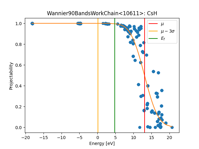
Exercise: Open the script and try to understand what it is doing.
As you can see, the protocol to choose \(\mu\) and \(\sigma\) ensures that the SCDM algorithm is applied to a density-matrix that includes (with a large weight) only those Kohn-Sham states that have a large projection on the manifold spanned by the PAOs.
Analyzing the provenance graph#
We begin by generating the provenance graph with
verdi node graph generate <PK>
where the PK corresponds to the workflow you have just run. You should obtain something like the following:
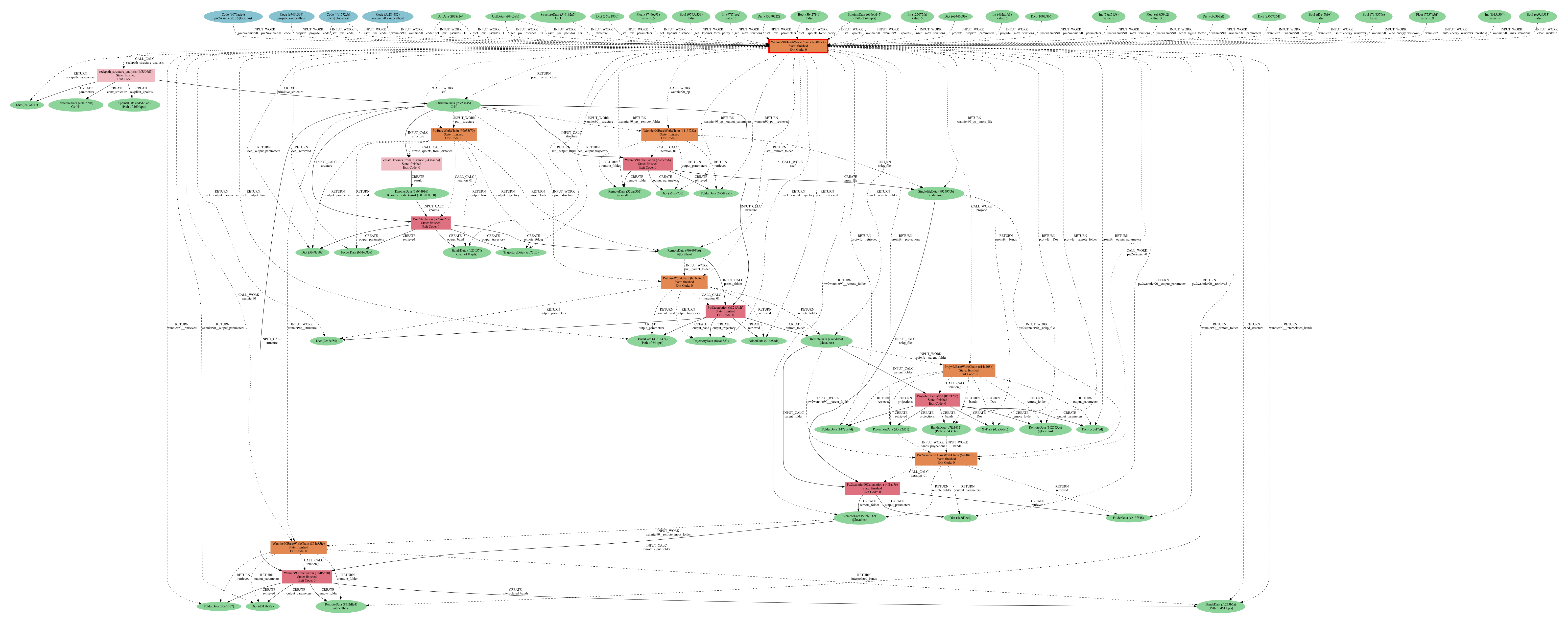
Provenance graph for a single Wannier90BandsWorkChain run. (PDF version
CsH.dot.pdf)#
As you can see, AiiDA has tracked all the inputs provided to all calculations (and their outputs), allowing you (or anyone else) to reproduce it later on.
(Optional) Maximal localisation and SCDM#
Try to modify the launch_wannier.py script to disable the MLWF
procedure in order to obtain Wannier functions with SCDM projections that are not maximally localised.
Hints: change the input parameters of the builder
params = builder["wannier90"]["wannier90"]["parameters"].get_dict()
params['num_iter'] = 0
builder["wannier90"]["wannier90"]["parameters"] = orm.Dict(params)
Exercise: Run the workflow for 1 or 2 materials of the dataset. Do you notice any difference when using or not the MLWF procedure? Which one gives better results? Do your results agree with the findings of the Automated high-throughput Wannierisation paper?
(Optional) Browse your database with the REST API#
Connect to the AiiDA REST API and browse your database! Follow the instructions that you find on the Materials Cloud website.
(Optional) More on AiiDA#
You now have a first taste of the type of problems AiiDA tries to solve, and you have seen how it is possible, thanks to the tools provided by AiiDA, to develop plugins and workflows to automate your research tasks, while preserving the full provenance and guaranteeing reproducibility of your results.
Here are some options for how to continue:
Continue with the in-depth tutorial and learn more about the
verdi,verdi shellandpythoninterfaces to AiiDA. There is more than enough material to keep you busy for a day. You can check for instance the dedicated AiiDA Tutorials.For advanced Linux & python users: try setting up AiiDA directly on your laptop. Note that AiiDA depends on a number of services and software that require some time to set up. Unfortunately, we will not have the time to help you solve issues related to your setup in a tutorial context, but you can refer to the AiiDA documentation and to the AiiDA mailing list.